For some Excel users, this change is less than ideal. The ribbon takes up a lot of space at the top of the window, and it can be difficult to find various menu options if you are accustomed to navigating in Excel 2003. But while there isn’t much that you can do about this switch, you can elect to minimize this ribbon so that it only displays when you click on one of the tabs at the top of the window. This frees up some extra space at the top of the program window, which will allow you to see more of your spreadsheet cells at once.
Minimize the Navigational Ribbon in Excel 2013
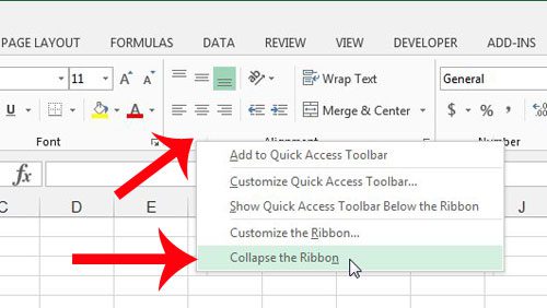
The steps in this article were performed in Microsoft Excel 2013. Earlier versions of Microsoft Excel can also minimize the ribbon using a similar method, but the screens will appear slightly different than those shown below. Following the guide below will change the settings in Excel 2013 so that the ribbon is not visible by default. However, you will see the ribbon when you click one of the tabs at the top of the window. The ribbon will then disappear once you click somewhere on the spreadsheet itself. You can unhide the ribbon by following these same steps. Step 1: Open Microsoft Excel 2013. Step 2: Right-click in an empty space on the ribbon, then click the Collapse the Ribbon option.
Note that this change will carry over after you close Excel. Would you also like to hide the formula bar that displays under the tabs? This article will show you how. After receiving his Bachelor’s and Master’s degrees in Computer Science he spent several years working in IT management for small businesses. However, he now works full time writing content online and creating websites. His main writing topics include iPhones, Microsoft Office, Google Apps, Android, and Photoshop, but he has also written about many other tech topics as well. Read his full bio here.