I use the freeze top row option a lot myself, especially when I’m working with a lot of data. While freezing the first row is useful when you have a header row that you want to keep visible, you might want to have more than one locked row at the top of your spreadsheet. Our tutorial below will show you how to lock a row in Excel, or how to lock multiple rows to make a large worksheet easier to manage.
How to Lock Multiple Excel Rows
Our article continues below with additional information on freezing cells in Excel 2013, including pictures of these steps. Using header rows in spreadsheet applications like Google Sheets or Microsoft Excel makes it much easier to identify information. But you might be wondering how to freeze multiple rows in Excel 2013 if you have several rows at the top of the spreadsheet that you want to keep visible. Creating a row of headings to identify your columns in an Excel spreadsheet is a popular way to organize data. But it can be difficult to remember which column contains which data as you scroll down and the headings row is no longer visible. Luckily, you can freeze the top row of your spreadsheet so that it remains frozen at the top of the sheet. But what if you have multiple rows that you want to keep visible at the top of the sheet instead? Fortunately, you can accomplish this as well, by taking advantage of the option to freeze a pane. Our tutorial below will show you how to freeze two or more of the top rows in your worksheet so that they remain fixed at the top of the sheet as you navigate further down the worksheet.
Freezing Two or More Rows at the Top of a Spreadsheet in Excel 2013 (Guide with Pictures)
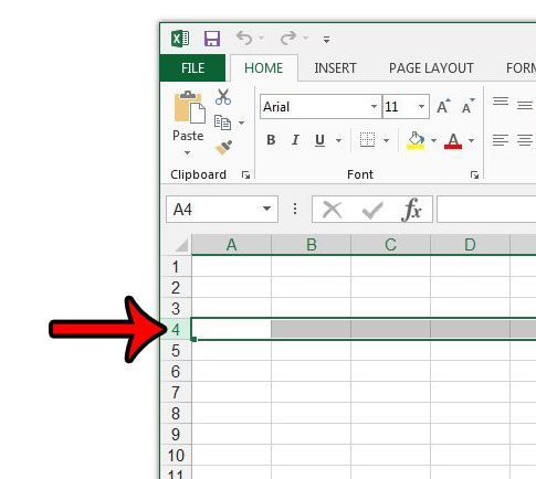
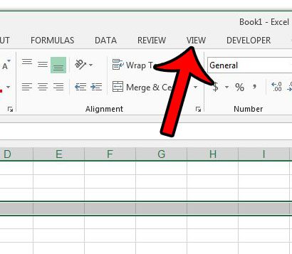
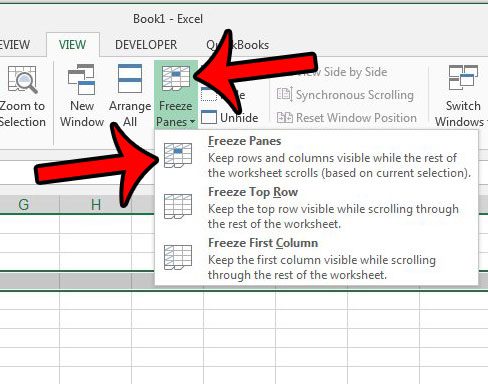
The steps in this guide will show you how to freeze the top three rows of a spreadsheet in Excel 2013. If you are working with Excel for Mac 2011, then read this article instead. We use three rows merely as an example. This same process can be applied to any number of the top rows in your spreadsheet. Now that you know how ot freeze multiple rows in your Excel worksheet you will be able to use this skill to make it easier to manage large sets of data in a worksheet. For example, we want to freeze the top 3 rows, so I have clicked row 4 in the picture above. If the drop-down menu says Unfreeze Panes instead, then you will need to click that first to remove the existing frozen pane, then click the Freeze Panes button.
How to Freeze Columns in Microsoft Excel
The same method in the section above will work if you want to freeze columns, too. Simply click on the column to the right of the columns that you want to freeze, then click the Freeze Panes button and select the Freeze Panes option. This can be a really useful thing to use if you are working on an Excel spreadsheet where you have your data headers in columns instead of rows. The next section of this article will discuss the steps that you need to complete when you are done working on your data and would like ot unfreeze the parts of your spreadsheet that are currently frozen.
How to Unfreeze Rows or Columns in Excel
If you accidentally freeze the wrong rows or columns, or if you receive a spreadsheet with unwanted frozen entities, then you can return to the View tab, click the Freeze Panes button, then choose the Unfreeze Panes option. While the ability to lock rows is helpful when you want to keep only rows with heading info in your worksheet visible at all times, other Excel users might be confused about why Excel has frozen cells or why you chose to lock specific rows to the top of the screen. Others may prefer to work with data in separate panes, or they might want to open multiple windows for the same spreadsheet and manage data that way instead.
Additional Info About the Excel Freeze Multiple Rows Tool
You can only freeze rows at the top of your spreadsheet, or columns at the left side of the spreadsheet. You aren’t able to freeze rows or columns in the middle, at the bottom, or at the right of the spreadsheet.If you need to keep a section of the spreadsheet visible and it isn’t at the top or left, then you may want to try the Split option instead. This can divide the sheet into different panes that can each be scrolled independently.You can tell that a row or column is frozen because there is a slightly darker line under the row, or the the right of the column.If you want to freeze the top row and the left column, click inside cell B2, choose the Freeze Panes option, then click Freeze Panes.
Do you need to print your Excel spreadsheet, but want to repeat the column headings on each page? Learn how to print the top row on every page in Excel 2013 to make it easier for your readers to identify which column a data cell belongs to.
Additional Sources
Luckily there is an option to freeze the leftmost column or a couple of the left columns, which is very similar to the freezing rows method we discussed above. Select the View tab at the top of the window, then click the Freeze Panes button. You can then select the Freeze First Column option. If you want to freeze more than one column then you will need to click the last column heading letter to the right of the last column that you want to freeze, then go to the View tab, click Freeze Panes, then click Freeze Panes again. So you can use this method to freeze first column data, or you can choose to free multiple columns instead. Once you have chosen the column(s) to freeze, they will remain locked to the left side of the sheet, while everything to the right of the last column you froze will be scrollable. Simply click the row below the last row that you want to keep in the top pane, then go to the View tab and click the Split button in the Window group of the ribbon. You will then be able to scroll in each pane independently without affecting the data in the other pane. Note that there is a gray line in the sheet that indicates where the split is located. If you no longer need your spreadsheet to be split like this, you can just go back to the View tab and click the Split button again to remove it. Working in multiple panes can take some getting used to, especially if someone is working on a sheet and isn’t expecting all the rows to stay locked to the screen. Choosing to freeze column ranges, or freezing multiple rows can be a little less confusing for people that aren’t used to managing Excel data like that. Simply go to the View tab, then click the New Window button. This will give you two separate windows, allowing you to simultaneously work on two different sets of data at the same time in the same worksheet. Luckily you can go to View > Freeze Panes > then select Unfreeze Panes to unlock the frozen panes and move your data around without having to worry about frozen rows or frozen columns. After receiving his Bachelor’s and Master’s degrees in Computer Science he spent several years working in IT management for small businesses. However, he now works full time writing content online and creating websites. His main writing topics include iPhones, Microsoft Office, Google Apps, Android, and Photoshop, but he has also written about many other tech topics as well. Read his full bio here.
You may opt out at any time. Read our Privacy Policy


