Ensuring that you have the right type of data in the cells of your Google spreadsheet becomes very important when you start using formulas to find or validate data. While it might seem trivial to type the same information correctly multiple times without making a mistake, typos and other errors are very common and can create problems when you are trying to perform automatic calculations on your data. One way to help with this situation is by taking a list of items that you want to use for your data, then creating a drop-down menu within a cell from that list. This allows individuals editing the spreadsheet to choose items from a list rather than type them manually, which is a method of data validation that can drastically reduce the amount of invalid data that appears in your spreadsheet. You can even customize the cell with the drop-down menu to show a warning if invalid data is entered, or to reject input entirely if the value entered is not on the list of items.
How to Create a Drop-Down List in Google Sheets
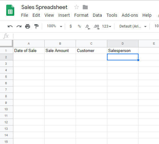
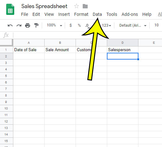
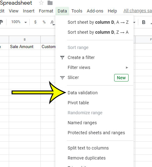
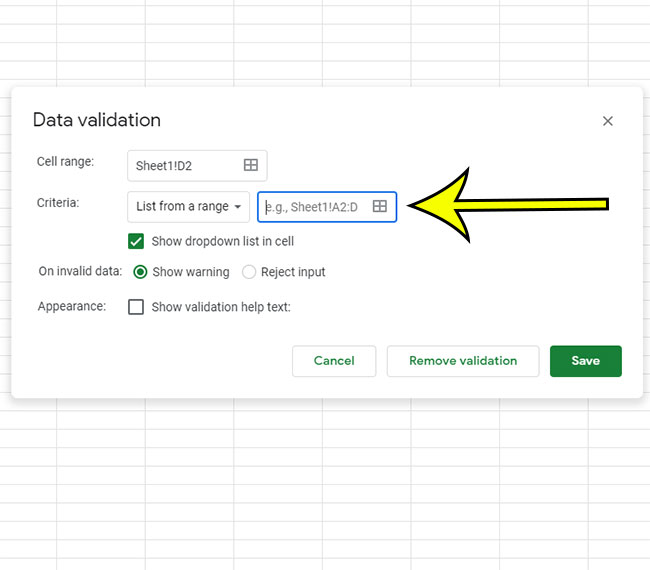
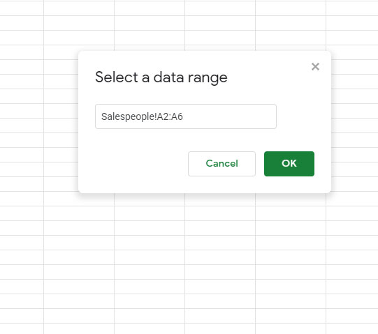
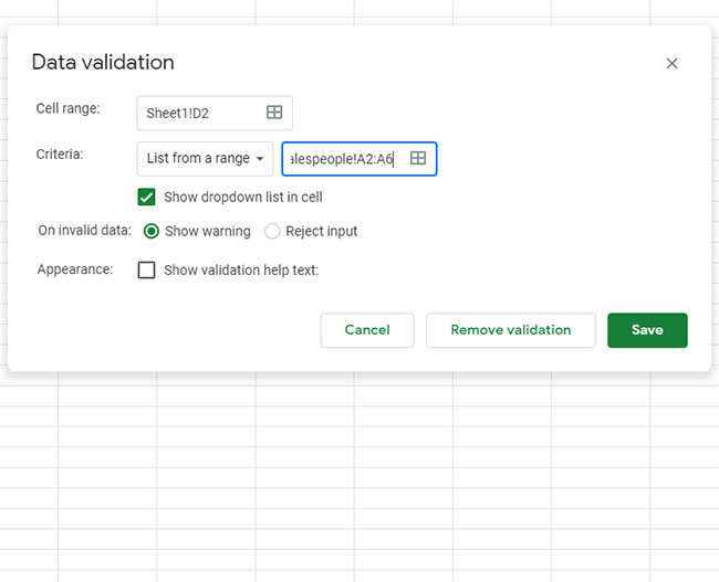
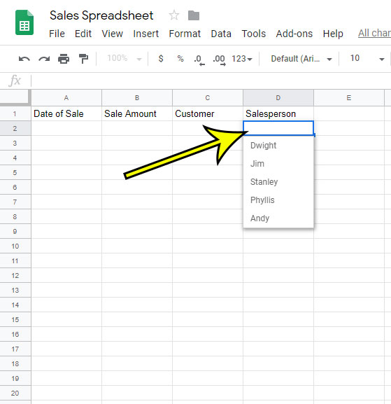
The steps in this guide were performed in the desktop version of the Google Chrome Web browser, but will work in other desktop browsers like Microsoft Edge or Mozilla Firefox. If you are familiar with creating drop-down menus in Microsoft Excel, then this process will feel fairly similar to that, although the exact method is slightly different. Step 1: Sign into your Google Drive at https://drive.google.com and open the Google Sheets file. Step 2: Select the cell or cell range in which you would like to create drop-down lists. You can even click the column letter at the top of the spreadsheet to select an entire column. Step 3: Click the Data tab at the top of the window. Step 4: Choose the Data validation option. Step 5a: Click the dropdown menu to the right of Criteria and choose the method that you want to use for your validation list. Step 5b (optional): If you selected the List from a range option, then click inside the cell to the right of the dropdown menu. Step 6 (optional): Find the cell range containing the cell values for your dropdown list, select them, then click the OK button. Step 7: Click the Save button. Note that there is an option on the menu shown in Step 7 above called Show validation help text. If you select that box you have the option of entering help text that you think will aid a spreadsheet user in using the dropdown list that you have created. Once the dropdown is in the cell, simply click the small down arrow in the cell to see the list of choices. If you click on one of those choices it will populate the cell with that value. You can remove a dropdown menu from a cell in Google Sheets if you right-click on the cell containing the dropdown, then choose the Data validation option at the bottom of the menu. You can then click the Remove validation button to remove the cell dropdown menu. Are there borders around some of the cells in your spreadsheet, but you would like to change them? Find out how to edit Google Sheets borders and apply a different color, or change one of several other characteristics of those cell borders. He specializes in writing content about iPhones, Android devices, Microsoft Office, and many other popular applications and devices. Read his full bio here.