But gridlines can be overridden by cell fill colors, so you may be looking for a way to regain those cell perimeters. This can be accomplished with borders. Our guide below will show you how to add borders to a selection of cells in your Excel 2013 spreadsheet. Before following the steps below, it is important to understand the difference between borders and gridlines in Excel 2013. They are two different things, and they can be used separately or together. Gridlines are applied to the entire spreadsheet at once, and you can elect to show them on the screen, or on a printed page. Borders can be set at the individual cell level, and will always print when they are active. You can read more about adding or removing gridlines in Excel 2013 if those seem to be closer to what you want.
How to Add Cell Borders in Excel 2013
Our article continues below with additional information on adding borders in Excel, including pictures of these steps.
How to Use Cell Borders in Microsoft Excel 2013 (Guide with Pictures)
The steps in this guide were performed in Microsoft Excel 2013, but will also work in many other versions of Excel, including Excel 2010, Excel 2016, and Excel for Office 365.
Step 1: Open your spreadsheet in Excel 2013.
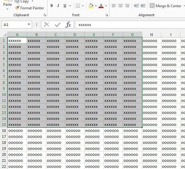
Step 2: Use your mouse to select the cells to which you would like to add borders.
You can select the cell or cells by either clicking on one cell and dragging your mouse, or you can select a range of cells by clicking on one cell then holding down the Shift key and clicking another cell at the end of the range in either the row or column.
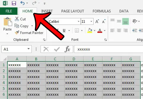
Step 3: Click the Home tab at the top of the window.
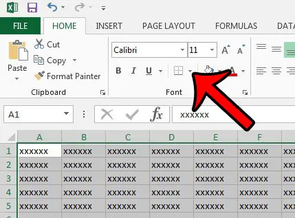
Step 4: Click the arrow to the right of the Borders button in the Font section of the ribbon.
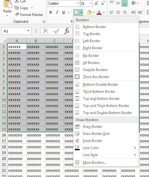
Step 5: Click the type of border that you want to apply to your selected cells.
There are a lot of border options on the drop down menu, but I find that I often use the “All Borders” option, as I want to apply full borders around all of the cells in my selection. Now that you have added borders to your cells, you can choose to change the color of those borders, if necessary.
Formatting Borders from the Format Cells Dialog Box
One other option for formatting cells in a spreadsheet involves an option on the right click menu. After you have selected your cells you can right click anywhere in the selection, then choose the Format Cells option. This is going to open the Format Cells dialog box. You can then select the Border tab at the top of this window, where you will see a handful of options. This includes things like adjusting the line style of your borders, as well as their color and which parts o the cells will have borders.
More Information on Cell Borders in Microsoft Excel
If your Excel worksheet has borders that you don’t want, then you can use a similar process to remove borders from your spreadsheet. Select the cells with the borders you would like to remove, then go to Home > Borders and choose the No Border option. You can quickly select every cell in your spreadsheet by selecting one of your cells, then using the keyboard shortcut Ctrl + A to select everything. You can then choose to apply or remove a border using the steps above, which will apply that effect to all of the cells in the worksheet. If you want to change the border setting for every sheet in your workbook then right click on one of the sheet tabs at the bottom of the window and choose the Select All Sheets option. Any border setting you choose will then be applied to every sheet in the workbook. It can be difficult to separate gridlines from cell borders because they seem so similar. Gridlines in a spreadsheet are displayed on the screen by default, and if you add borders to your cells they will follow the same row and column borders as the gridlines. But gridlines don’t print by default, (though you can print them by checking the option next to Print under Gridlines on the Layout or Page Layout tab), while borders so. You can also easily change the border color, which I have found to be one of the main reasons that I ever elect to use borders in Excel. There is one weird interaction with borders that you should be aware of. It’s possible to make cell borders white, which can cause a lot of headaches when you are trying to work with gridlines. Since cell borders are displayed “above” your gridlines, it’s possible for you to have white borders on your cells which prevent the gridlines from being shown or printed. If you have an issue with getting gridlines to display or print, try turning off the borders completely to see if that helps.
Conclusion
Being able to add borders in Excel 2013, or conversely, being able to remove them, can be a handy tool to have when you are running into unexpected issues with the display or printing of your cells. Excel is a notoriously difficult application to use when you need to print a spreadsheet, which is one of the reasons that many people have migrated to Google Sheets. The Google version of the spreadsheet application is powerful, easy to use, and can be used in a Web browser or on a smartphone effectively.
Additional Sources
After receiving his Bachelor’s and Master’s degrees in Computer Science he spent several years working in IT management for small businesses. However, he now works full time writing content online and creating websites. His main writing topics include iPhones, Microsoft Office, Google Apps, Android, and Photoshop, but he has also written about many other tech topics as well. Read his full bio here.
You may opt out at any time. Read our Privacy Policy


